QUANTUM ESPRESSO:Wannier90拟合
从bandfat数据分析,在带隙附近的能带主要由C原子sp2和pz轨道贡献
进行wannier计算的步骤如下:
-
用pw.x运行‘scf’计算,使用修改版的
PW/src/summary.f90重新编译的pw.x将可以输出能够用于wannier90.x输入文件的结构参数:1 2 3 4 5 6 7 8 9 10 11 12 13 14
Begin Write cell and positions for Wannier90.x begin unit_cell_cart Bohr 4.8484202 0.0000000 0.0000000 0.0000000 28.3458919 0.0000000 0.0000000 0.0000000 28.3458919 end unit_cell_cart begin atoms_cart Bohr C -0.0000026 14.1729459 14.1729459 C 2.3890085 14.1729459 14.1729459 end atoms_cart End Write cell and positions for Wannier90.x
-
用pw.x进行’nscf’计算,需要列出所有k点的坐标,和权重,使用kmesh.pl生成。注意修改
nbnd,使得其包含要拟合的能带,通过fatband的结果来看需要采用多少条能带。1 2 3 4 5 6 7 8 9
cp scf.in nscf.in calculation = 'nscf' nbnd = 22 !K_POINTS{automatic} !1 1 200 0 0 0 kmesh.pl 1 1 200 >>nscf.in pw.x <nscf.in>nscf.out
-
运行wannier90.x -pp (预处理pre-process,或在输入文件内写postproc_setup = .true.)生成seedname.nnkp。该过程比较快,可以在主节点直接运行。
使用命令:1
awk '/Begin Write/,/End Write/' scf.out|awk '/begin unit/,/end atoms/'>>carbyne.win
-
构建输入文件carbyne.win
1
2
3
4
5
6
7
8
9
10
11
12
13
14
! System
begin unit_cell_cart
Ang
 10.000000   0.000000   0.000000
  0.000000  10.000000   0.000000
  0.000000   0.000000   2.56551169
end unit_cell_cart

begin atoms_cart
Ang
C       5.0000000000       5.0000000000       0.0000000000
C       5.0000000000       5.0000000000       1.2640744811
end atoms_cart
-
添加k-points信息 note: dis_win_max的值要根据fatband的结果进行设置,不能随意设置的无限高或者不设置,这样会导致得到的wannier函数很难局域化。Wannier函数局域化的条件要求,(1)wannier函数spread较小,一般每一个wannier函数小于1.0(Ang^2),(2)wannier函数Maximum Im/Re Ratio 的值小,一般应该小于0.001,在wannier函数局域,但是wannier函数虚部比较大时,一般是由于
nbnd设置的太少或者太多,当太少时,导致不能projector函数没有包含在所计算的能带中,当太多时,能带中包含了其他的具有相类似性质的投影轨道,导致解纠缠时会很慢收敛,并导致得到解纠缠得到的轨道不合适。在graphene中就是由于nbnd设置的太大导致的这个问题,设置为56时可以得到局域实数的WFs。最好是nbnd的设置,使得在fatband时,正好有相同的投影能带数。(3)Wannier函数拟合得到的能带结构能够与DFT计算得到的能带结构相同,这一条件必须满足。 在画wannier函数时,最好选择cube格式进行输出,采用xcrysden输出的结果采用VESTA画图可能会有问题。
1
2
3
4
  echo "mp_grid = 1 1 200">>${seedname}.win
  echo "begin kpoints">>${seedname}.win
  kmesh.pl 1 1 200 wannier >>${seedname}.win
  echo "end kpoints">>${seedname}.win
- 添加wannier拟合参数
1
2
3
4
5
6
7
8
9
10
11
12
13
14
15
16
17
18
19
20
21
22
23
24
25
26
27
28
29
30
31
32
33
34
35
36
37
38
39
40
41
42
43
44
45
46
47
48
49
50
51
52
53
54
55
56
57
58
 !System
 num_wann  = 4
 num_bands = 20

 !Projection
 begin projections
 !! Atom-centred px,py orbitals
 !C : px;py
 !! Bond-centred px,py-orbitals
 f=0.5,0.5,0.25:px;py
 f=0.5,0.5,0.75:px;py
 end projections

 !Job Control
 exclude_bands : 1-2
 translate_home_cell = .true.
 !restart =

 !disentanglement
 dis_win_min  = -10.0
 !dis_win_max  = 12.0
 dis_froz_min = -11.0
 dis_froz_max = -0.5
 dis_num_iter = 1000
 dis_mix_ratio= 0.5
 dis_conv_tol = 1.0E-10
 dis_conv_window = 5

 !Wannierise
 num_iter = 10000
 conv_tol = 1.0E-10
 conv_window     = 10
 guiding_centres = .true.

 !Post-Processing
 !restart = plot
 wannier_plot = .true.
 wannier_plot_format = cube
 wannier_plot_mode   = crystal
 wannier_plot_supercell = 1 1 3
 translate_home_cell = .true.

 bands_plot = .true.
 bands_num_points = 100
 bands_plot_format = gnuplot
 begin kpoint_path
     M 0.0 0.0 -0.5 G 0.0 0.0 0.0
     G 0.0 0.0  0.0 M 0.0 0.0 0.5
 end kpoint_path

 fermi_surface_plot = .true.
 fermi_surface_num_points = 100
 fermi_energy = -5.262

 write_hr=.true.
 write_rmn=.true.
 write_tb=.true.
 !end plot
- 运行wannier90.x -pp seedname
NOTE: 其结果中包含有初始指定的projections函数(以alat为单位): ! convert wannier center in cartesian coordinates (in unit of alat)
-
-
Run pw2wannier90 to compute the overlap between Bloch states and the projections for the starting guess (written in the seedname.mmn and seedname.amn files). 该过程比较慢,最好在计算节点完成。
pw2wannier90.x < pw2wan.in > pw2wan.out输入文件
pw2wan.in如下:1 2 3 4 5 6 7 8 9
&inputpp outdir = './outdir' prefix = 'carbyne' seedname = 'carbyne' spin_component = 'none' write_mmn = .true. write_amn = .true. write_unk = .true. /
要在后续wannier90.x使用plot画MLWF函数,需要设置
write_unk=.true.NOTE可能会遇到报错
1
2
3
4
 %%%%%%%%%%%%%%%%%%%%%%%%%%%%%%%%%%%%%%%%%%%%%%%%%%%%%%%%%%%%%%%%%%%%%%%%%%%%%%
 Error in routine  fft_type_set (6):
 there are processes with no planes. Use pencil decomposition (-pd .true.)
 %%%%%%%%%%%%%%%%%%%%%%%%%%%%%%%%%%%%%%%%%%%%%%%%%%%%%%%%%%%%%%%%%%%%%%%%%%%%%%
需要使用
mpirun -np $NP pw2wannier90.x <pw2wan.in> pw2wan.out并行计算,并且$NP太大时会导致部分核分配不到平面波,需要适当减小\$NP的值 -
Run wannier90 to compute the MLWFs.
mpirun -np 28 wannier90.x seedname
并在seedname.win中添加plot部分1 2 3 4 5 6 7 8 9 10 11 12 13 14 15 16 17 18 19 20 21 22
!restart = plot wannier_plot = .true. wannier_plot_format = xcrysden wannier_plot_supercell = 1 1 3 bands_plot = .true. bands_num_points = 100 bands_plot_format = gnuplot begin kpoint_path M 0.0 0.0 -0.5 G 0.0 0.0 0.0 G 0.0 0.0 0.0 M 0.0 0.0 0.5 end kpoint_path fermi_surface_plot = .true. fermi_surface_num_points = 100 fermi_energy = -5.262 write_hr=.true. write_rmn=.true. write_tb=.true. !end plot
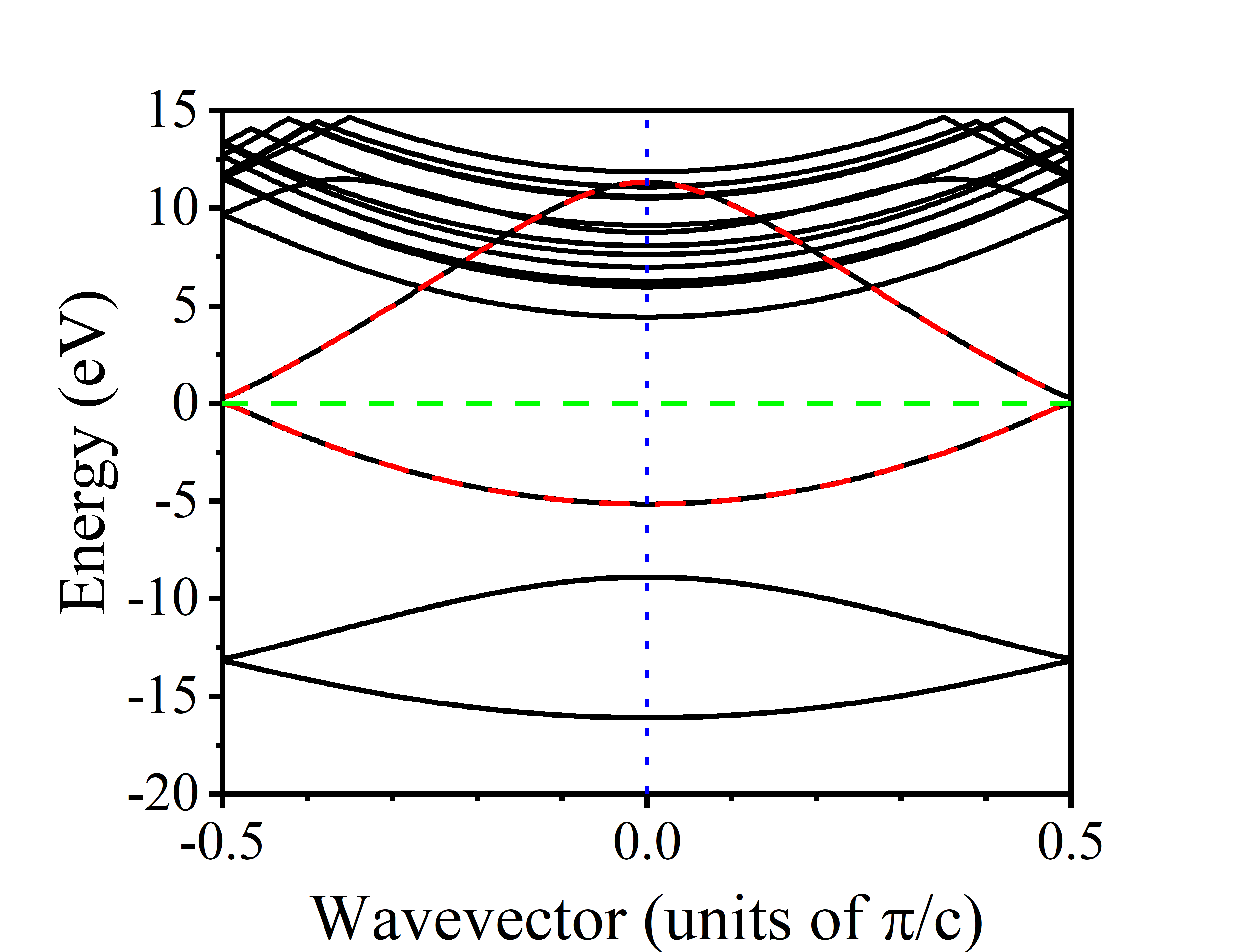
计算得到的wannier插值的能带图如下:
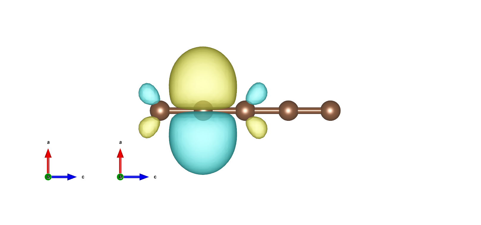
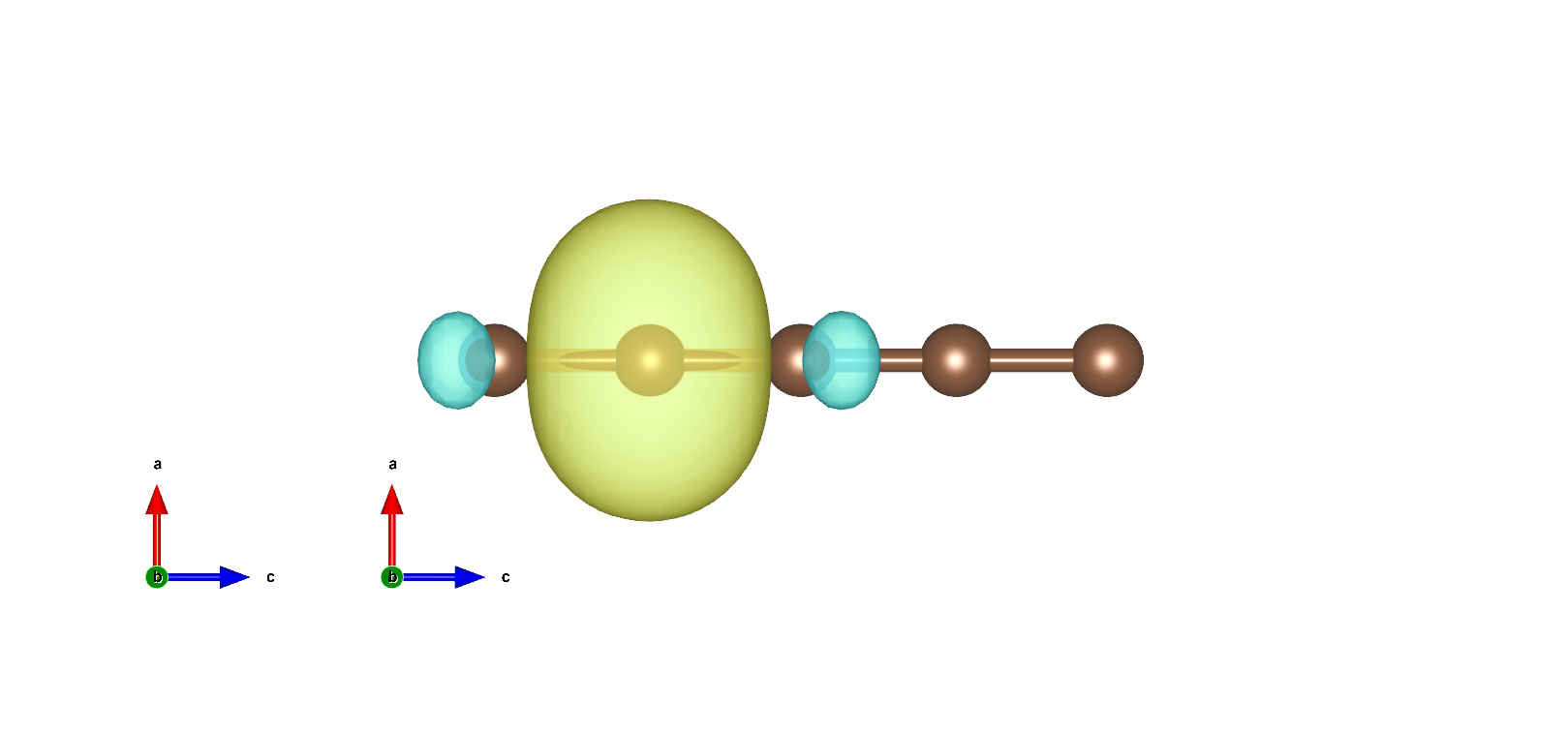
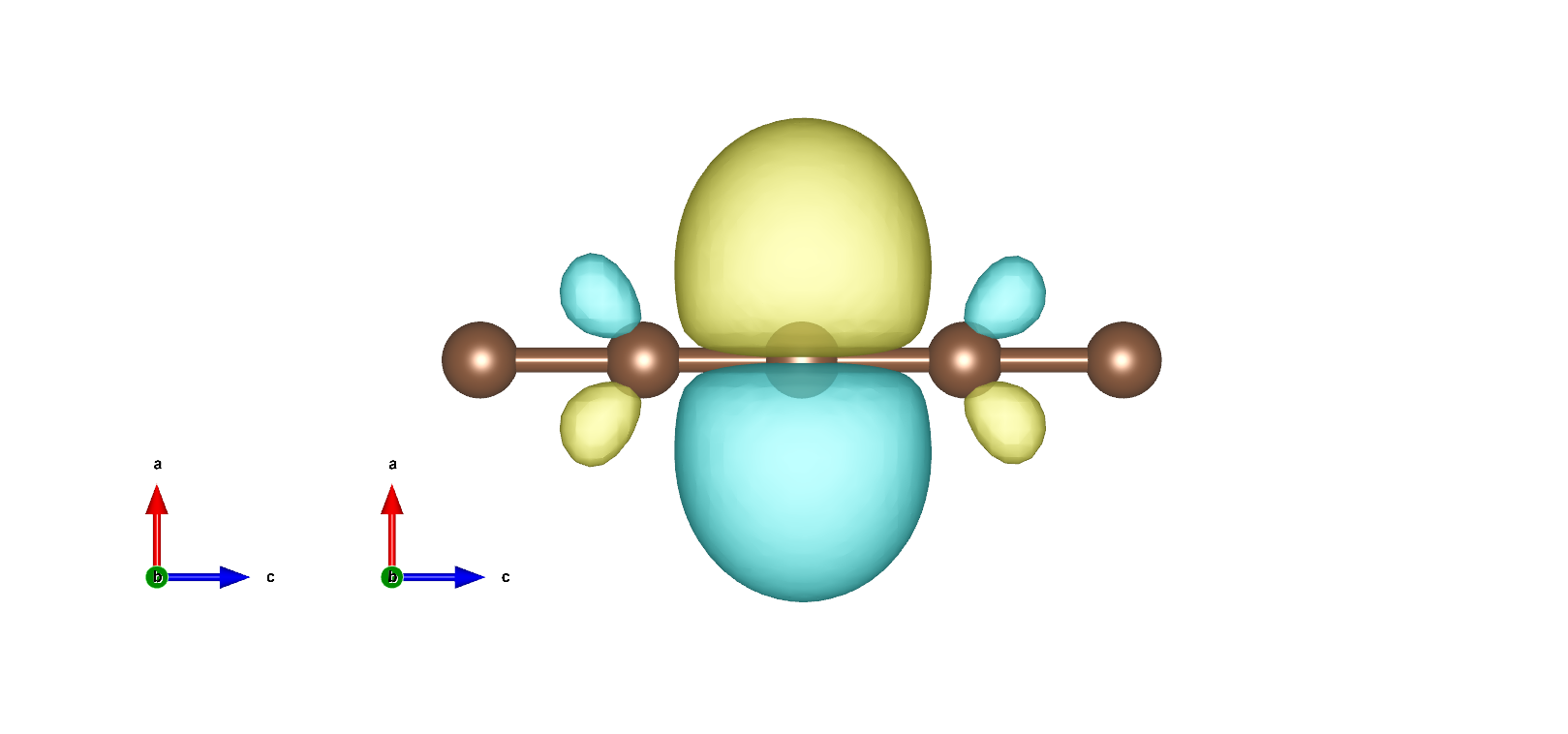
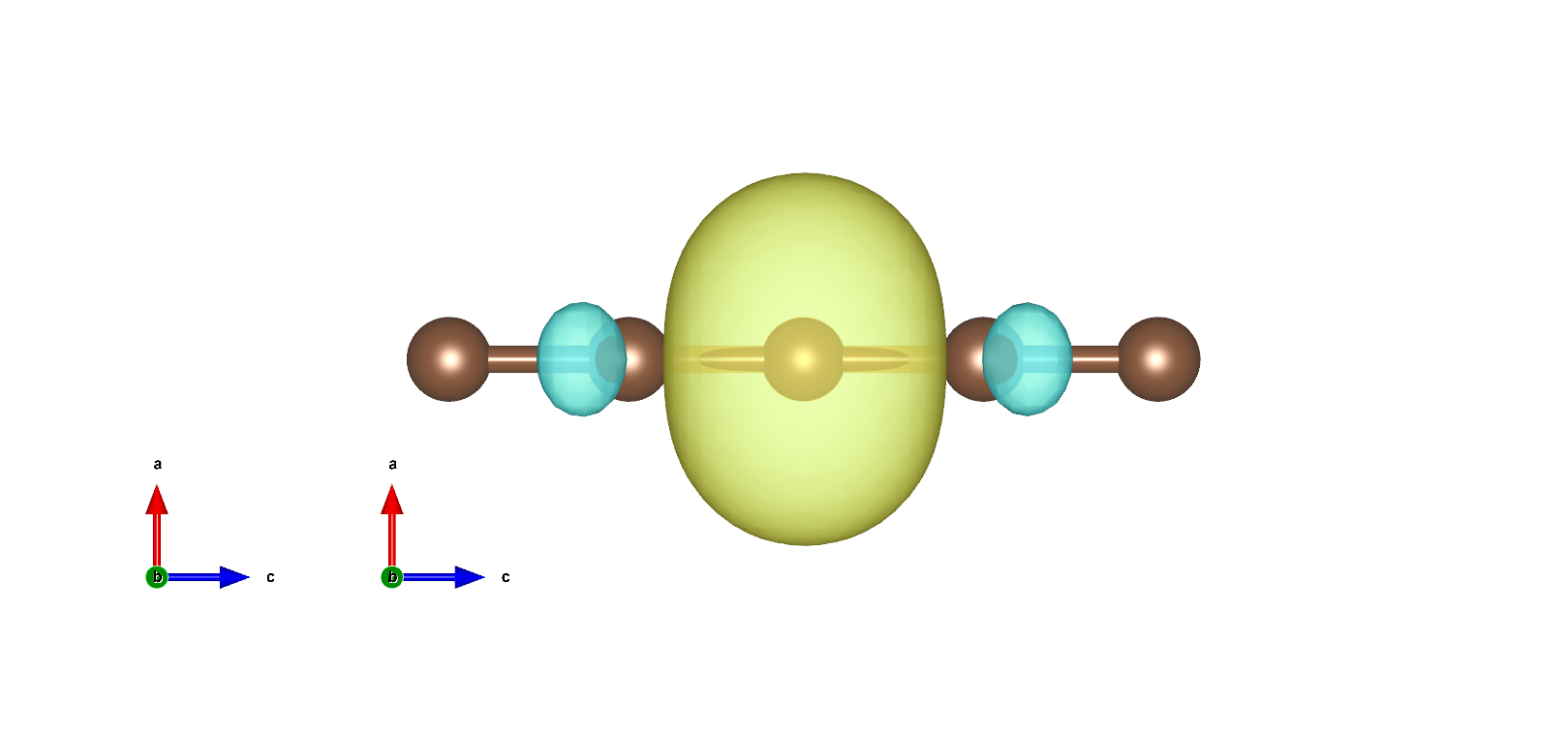
MLWF如下: